1. Pushing and pulling
In this question we will be deriving the continuum movement equation behind the discretised movement schema presented in Figure 1. Specifically, there is a local spatially dependent rate, \(r\), which pushes the particles out of their current location to a neighbouring location. Namely, the rate function is evaluated at the same position as the population that it is acting on, e.g. the rate of jumping from \(x_i\) (to either \(x_{i-1}\) or \(x_{i+1}\)) is \(r(x_i)u(x_i)\).
Further, there is a non-local spatially dependent rate, \(s\), which pulls the particles from their current location to a neighbouring location. Namely, the rate function is evaluated at the position the population is jumping to, e.g. the rate of jumping from \(x_i\) to \(x_{i+1}\) is \(s(x_{i+1})u(x_i)\).
We begin as in the lecture notes, namely, consider an infinite one-dimensional interval that is discretised into points of width \(\Delta x\). Each population is centred at a point \(x_i\) where \(i\) is an integer label and \(x_{i+1}=x_i+\Delta x\). The moving population, \(u\), is labelled by both its spatial location and time during its evolution, \(u(x_i,t)\). For simplicity, \(u(x_i,t)=u_i\). Members of each population are able to transition to their neighbours at the rates presented in Figure 1.
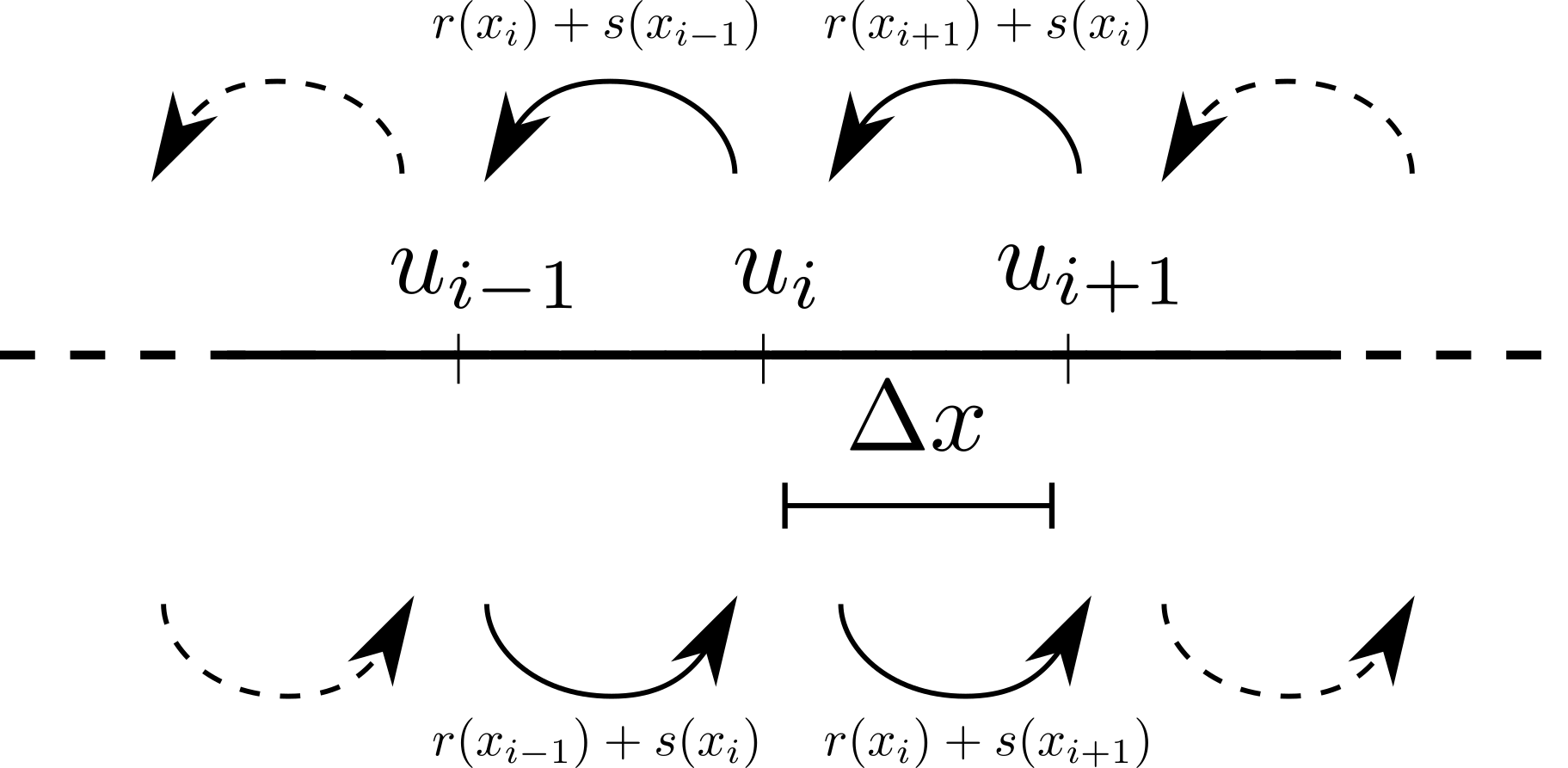
The push and pull movement schematic.
Why can we ignore boundary conditions and just simply construct equations for \(\dot{u}_i\)?
Using the Law of Mass Action and Figure 1 show that the expression for \(\dot{u}_i\) is
\[\dot{u}_i=u_{i+1}[ r(x_{i+1})+s(x_i) ]-u_i[ s(x_{i-1})+2r(x_i)+s(x_{i+1})]+u_{i-1}[ r(x_{i-1})+s(x_i) ]. \tag{1}\]
Expand equation (1) up to second order in \(\Delta x\). Remember you will have to use Taylor series to expand \(u\), \(r\) and \(s\). You should find the first-order terms all cancel.
Suppose we want to take the limit of \(\Delta x\rightarrow 0\) and recover a non-trivial finite limit. How should \(r\) and \(s\) scale with \(\Delta x\)? Namely, what values of \(\alpha\) and \(\beta\) provide a finite limit when we set \(r(x)=R(x)\Delta x^\alpha\) and \(s(x)=S(x)\Delta x^\beta\)?
Substitute \(r(x)=R(x)\Delta x^\alpha\) and \(s(x)=S(x)\Delta x^\beta\) into the equations and show that the limiting equation is then
\[\frac{\partial u}{\partial t}=\frac{\partial }{\partial x}\left(\frac{\partial u}{\partial x}S-u\frac{\partial S}{\partial x}\right)+\frac{\partial^2 \left(uR\right)}{\partial x^2}. \tag{2}\]
What happens in the specific case that \(r=s\)?
2. Travelling waves
Foxes are territorial animals, unless they have rabies, in which case they undergo random walks away from their home range. Rabies is fatal in foxes.
Justify the following equations as a model of this situation,
\[\begin{align} \frac{\partial I}{\partial t}=&D\frac{\partial^2 I}{\partial x^2}+\alpha IS-\beta I,\tag{3}\\ \frac{\partial S}{\partial t}=&-\alpha IS+rS\left(1-\frac{S}{K}\right), \tag{4} \end{align}\]
where the populations \(S\) and \(I\) and the positive constants \(D\), \(\alpha\), \(\beta\), \(r\) and \(K\) should be interpreted.
Non-dimensionalise the system to give
\[\begin{align} \frac{\partial u}{\partial \tau}=&\frac{\partial^2 u}{\partial X^2}+uv-\mu u,\tag{5}\\ \frac{\partial v}{\partial \tau}=&-uv+\gamma v\left(1-v\right), \tag{6} \end{align}\]
where \(\gamma\) and \(\mu\) should be defined in terms of \(D\), \(\alpha\), \(\beta\), \(r\) and \(K\).
What are the spatially uniform steady states of system (5)-(6)? Explain what each steady state represents.
Conclude why \(0<\mu<1\) must occur if a non-zero infective population is to constantly exist.
Convert equations (5) and (6) to moving wave coordinates. Namely substitute \(z=X-c\tau\), where we assume that \(c\) is a positive constant.
Look for a travelling wave solution that does not change shape over time. Linearise far ahead of the wave front, where the population is fully susceptible and the infection has not yet arrived. Namely, consider expansions of the form
\[\begin{align} u=&\epsilon_1\exp(\lambda z),\tag{7}\\ v=&1+\epsilon_2\exp(\lambda z). \tag{8} \end{align}\]
Show that if a travelling wave exists the wave speed must satisfy \(c\geq 2 \sqrt{1-\mu}\).
3. Simulating diffusion
Matlab has inbuilt codes that allow you to simulate one-dimensional partial differential equations easily. However, in this example, we will show that the discretised approximation also produces a good approximation to the diffusion equation.
From the notes we saw that the diffusion equation,
\[\frac{\partial u}{\partial t}=D\frac{\partial^2 u}{\partial x^2}, \tag{9}\]
with zero-flux boundary conditions can be discretised into the following form
\[\begin{align} \frac{\partial u_1}{\partial t}=&du_{2}-du_1,\tag{10}\\ \frac{\partial u_i}{\partial t}=&du_{i-1}-2du_i+du_{i+1},\tag{11}\\ \frac{\partial u_N}{\partial t}=&du_{N-1}-du_N. \tag{12} \end{align}\]
where \(d=D/\Delta x^2\) is the ratio of the diffusion constant and the discretised domain’s individual box size. Equations (10)-(12) form a large coupled system of ODEs. Thus, we can use ode45 to simulate the system. This is what the code below does.
Note that in this code we plot the solution in two different ways. One way (lines 32-40) is the standard space concentration graph. Namely, we fix a time and plot the solution at the time. The second way (lines 22-29) involves creating a space-time plot which shows all of the solution at once and uses the colour channel to plot the concentration as a surface.
Try decreasing
dxin line 9. This should make the solution smoother.Try making an animation of the solution over time by using a
forloop, which increments the time value of the solution and creates a plot at each time step.
%% Ensure we start from a blank slate
clear all
close all
clc

%% Initialise variables
fs=15; % Set fontsize

dx=0.1; % Set box size
T_steps=1000; % Set number of time steps over which the solution is evaluated
x=0:dx:1; % Create the spatial discretisation
N=length(x); % Defines how many ODEs there will be
t=linspace(0,1,T_steps); % Create time series
ICs=zeros(N,1); % Initialise initial condition to be a zero vector
ICs(1)=2; % Put a value of 2 in the first box as the initial condition

%% Solve the N coupled ODEs
[t,y]=ode45(@(t,y)ODE(t,y,N,dx),t,ICs);


%% Plot space-time graph
figure('units','normalized','position',[0 0 1 1/3])
subplot(1,2,1)
pcolor(x,t,y)
shading interp
xlabel('Space')
ylabel('Time')
colorbar
set(gca,'fontsize',fs)

%% Plot spatial profile over a number of time points
subplot(1,2,2)
plot(x,y(1,:))
hold on
plot(x,y(floor(T_steps/10),:))
plot(x,y(T_steps,:))
legend('$t=0$',['$t=$ ',num2str(t(floor(T_steps/10)))],['$t=$ ',num2str(t(floor(T_steps)))])
xlabel('Space')
ylabel('$u$')
set(gca,'fontsize',fs)


function dydt=ODE(t,y,N,dx)
D=0.1; % Diffusion rate

% First and last box are set with Neumann boundary conditions
dydt(1,1)=D/dx^2*(-y(1)+y(2));
dydt(N,1)=D/dx^2*(y(N-1)-y(N));

% Fill in all other vector values
for i=2:N-1
    dydt(i,1)=D/dx^2*(y(i-1)-2*y(i)+y(i+1));
end

end
Exam Revision
4. Nonlocal diffusion
Consider a population moving on a discretised infinite domain that is able to jump to one of its three neighbouring boxes with rate \(d\) (see Figure 2).
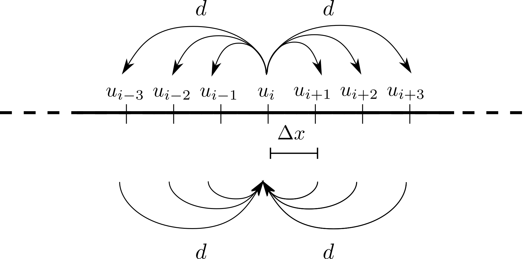
Nonlocal motion. Note that the population can jump to any of its neighbouring three populations. This is true for all boxes, but only movement to and from population \(i\) is shown for clarity.
Before we begin the question, what PDE do you think is behind this system?
Write down the ODE for \(u_i\).
Using Taylor series expand the \(u_i\) ODE in terms of \(\Delta x\).
How should \(d\) scale with \(\Delta x\) to produce a nonsingular and nontrivial equation?
Derive the PDE limit of the ODE when \(\Delta x \rightarrow 0\).
Does the PDE you derived match your intuition?
5. Nonlinear travelling wave
Consider a population of cells on an infinite one-dimensional domain that undergoes logistic growth, but whose diffusion depends linearly on their density,
\[\frac{\partial u}{\partial t}=\frac{\partial }{\partial x}\left(u\frac{\partial u}{\partial x}\right)+u(1-u). \tag{13}\]
The boundary conditions are \(u(-\infty,t)=1\) and \(u(\infty,t)=0\) and the initial condition is such that the wave has not entered into the positive \(x\)-axis \(u(x,0)=0\) for all \(x>0\), i.e. the population is invading an empty space.
Convert the equation into travelling wave coordinates, \(z=x-ct\), where \(c>0\).
Suppose there is a travelling wave solution with stationary profile, which is constrained to have the form \(u_z=c(u-1)\). Show that there is an exact solution for one value of the wave speed, c, which you should state.
By solving \(u_z=c(u-1)\) subject to the boundary conditions \(u(-\infty,t)=1\) and \(u(A,t)=0\) and initial conditions \(u(x,0)=0\) show that such a solution must be piecewise continuous i.e.
\[u=\left\{\begin{array}{c} u(z) \textrm{ for } z<A\\ 0 \textrm{ for } z\geq A\\ \end{array}\right. \tag{14}\]
where \(u(z)\) and \(A\) should be found.
Sketch what the travelling wave solution will look like.