1 Michaelis-Menten Enzyme dynamics

Enzymes are biological molecules (typically proteins) that significantly speed up the rate of virtually all of the chemical reactions that take place within cells. They are vital for life and serve a wide range of important functions in the body, such as aiding in digestion and metabolism.

In 1913 Leonor Michaelis and Maud Menten proposed a mathematical model of how enzymes work. The process involves an enzyme, E, binding to a substrate, S, to form a complex, C, which in turn releases a product, P, regenerating the original enzyme. This may be represented schematically as (see Figure 1)

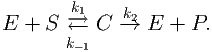(1)

1.

Use the Law of Mass Action to right down the ODE formulation of the dynamics. The initial conditions are

(2)

2.

Show E + C =constant= E₀.

3.

Why can we ignore the equations for Ṗ and Ė? Specifically, show that we only need to consider the equations

Ṡ	= -k1(E0 - C)S + k-1C,	(3)
Ċ	= k1(E0 - C)S - (k-1 + k2)C.	(4)

4.

Use the following scales to non-dimensionalise the equations

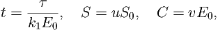(5)

to produce the following system

	= -u + (u + K - λ)v,	(6)
ϵ	= u - (u + K)v.	(7)

What are ϵ, λ and K? Show that ϵ, λ and K are non-dimensional.

5.

What are the initial conditions?

6.

Suppose E₀ is much less than S₀ (what does this mean?) and so let ϵ → 0. Show that we can write v as a function of u, which simplifies the du∕ dτ equation to

(8)

This is known as the system on the ‘outer’ time-scale.

7.

Substitute the time scale σ = τ∕ϵ into equations (6) and (7). Rearrange the system and, once again, let ϵ → 0. You should be able to show that the solution of the system is

u(σ)	= 1,
v(σ)	= .	(9)

This is known as the system on the ‘inner’ time-scale.

In questions 7-6 you have done a multiple scales simplification of the Michaelis-Menton problem. Namely, the whole equation is hard to solve. However, we can solve for what the equation looks like for small time, σ (question 7) and we can solve for what the equations looks like for large time, question (6). In the computation question, which is next, we check these approximations.

2 Computer simulation

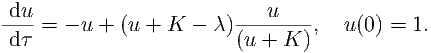
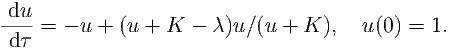
Let K = 2, λ = 1 and ϵ = 0.001. Simulate

	= -u + (u + K - λ)v, u(0) = 1	(10)
ϵ	= u - (u + K)v v(0) = 0.	(11)

and

(12)

with v = u∕(u + K) over the time t ∈ [0,20]. How well do these curves approximate each other?

3 Spruce budworm

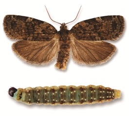
Spruce budworm (see Figure 2) are preyed upon by spiders, miscellaneous insects, and birds. A model for their population size, N is given by

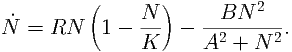(13)

1.

What does each term in the equation mean?

2.

Describe, with a sketch, three properties of the predation term

(14)

Hint: consider low, medium and high values of N.

3.

Non-dimensionalise the equation to give the form

(15)

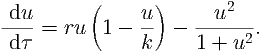
What are the scales of the population and time in terms of A, B, K and R? What are the parameters r, k in terms of A, B, K and R?

4.

Show the population and time scales have the right dimension. Show that r and k are dimensionless.

4 Spruce budworm population stability

You can find more about the spruce budworm population equation and an online applet that allows you to simulate the system quickly and easily at the following website:

(16)

The above website may aid in the following questions as we are going to consider the steady states of

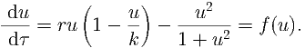(17)

We could solve f(u) = 0, however, this leads to a cubic in u. This can be solved, but it is not very fun. Instead, we are going to consider sketches of the system.

We could sketch f(u), directly, and draw arrows on the diagram, such that u is increasing if f(u) > 0 and u is decreasing if f(u) < 0. This will immediately tell us how many stationary states there are and inform us of their stability. We will do this towards the end of this question, however, going straight into the full sketch may cause us to miss certain cases, as we have two parameters, r and K, to worry about. However, if you feel confident shoot straight to question 3.

Critically, the following questions only deal with sketches. Thus, you do not have to be exactly accurate in your plotted values. We are just need to provide the general shape of the curve. This means little, if any, calculation should be required. Namely, an exact analytical result is not required, only approximate sketches backed up by logical thought.

1.

By inspection u₀ = 0 is always a steady state of f(u) (make sure you understand why). Instead of considering f(u) let us consider the two functions

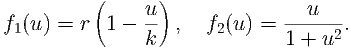(18)

Sketch f₂ on three different axes. Fix the value of r∕k to be greater than zero (say r∕k = 0.05), but allow r to vary (with k being defined by, say, k = 0.05∕r). Sketch on these three different plots f₁ for different values of r, namely consider r small, medium and large¹

2.

Draw on your above diagrams regions where f₁ > f₂ and regions where f₂ > f₁.

3.

Noting that a steady state, u′, satisfies

(19)

use your sketches of f₁ and f₂ to plot three situations of f(u).

4.

You should be able to show that (depending on the value of the parameters) there can be as few as two steady states and as many as 4 steady states. Name the four steady states 0 = u₀ < u_- < u_s < u₊, in the obvious way. Specify on your diagrams these four steady states. The middling value of r sketch is given in Figure 3.

---

Figure 3: Plots of f for a middling value of r.

---

5.

Use each sketch of f(u) to state the stability of each steady state, u₀, u_-, u_s and u₊ (when they exist).

6.

Does the system exhibit hysteresis? To solve this follow these steps:

(a)

start with a low value of r, such that only u₀ and u_- exist. Suppose we start with a small initial condition, where do you evolve to?

(b)

increase r until u₀, u_-, u_s, u₊ all exist, what happens to the point you evolve to?

(c)

increase r further until only u₀ u₊ exist, what happens to the point you evolve to?

(d)

decrease r until u₀, u_-, u_s, u₊ all exist, what happens to the point you evolve to?

(e)

is the point you evolve to in step 6b the same as the point you evolve to in step 6d? Use this to answer the original question.

Exam revision

5 Stability of a one variable system

Consider the following equation

(20)

1.

What are the steady states?

2.

Linearise around each steady state. Which steady states are stable and which are unstable? Why can you not categorise the stability of u = 1 and u = 2?

3.

Sketch the phase plane (u,) and show that your linear analysis tallies with the stability information gained from the sketch.

4.

Use the sketch to categorise the stability of u = 1 and u = 2.

6 Infections

The interaction dynamics of any disease can be understood by modelling three sections of the population: the susceptible population, S; the infected population, I and the recovered population, R. They interact through the following rules:

• whenever a susceptible agent interacts with an infective agent the result is two infective agents at a rate r₁;
• the infected population recovers at a rate to proportional the size of the infected population, the rate of proportionality is r₂.

Finally, suppose that the initial densities of the susceptible and infectives are S₀ and I₀, respectively, and that there are no initially recovered people.

1.

Convert the above rules into interaction equations.

2.

Use the Law of Mass Action to convert the interaction equations into ODEs.

3.

Show that S + I + R = constant = S₀ + I₀. What does this mean?

4.

What are the dimensions of S, I, R, Ṡ, İ, Ṙ, r₁ and r₂ in terms of density and time?

5.

Let S = [S]S′, I = [I]I′, R = [R]R′ and t = [t]t′ where the bracketed variable is the dimensional part and the primed variable be the non-dimensional part. Further, suppose we non-dimensionalise the system as

	= S′I′, S′(0) = S′0,
	= S′I′- I′, I′(0) = I′0,
	= I′, R′(0) = 0,

where the ˙ symbol now stands for d∕ dt′. What are the scales [S], [I], [R] and [t] in terms of r₁ and r₂? Show that they have the right dimension, i.e. [S] has the same dimension as S, as specified in question 4.

6.

What are the forms of S′₀ and I′₀ in terms of r₁, r₂, S₀ and I₀?

7.

By integrating

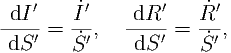(21)

find expressions for I′(S′) and R′(S′). Do not forget about the initial conditions.